Tutorials
Short Tutorial in the Retention Class.
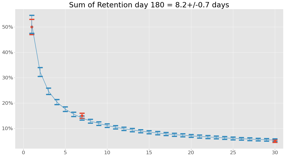
Let’s import the class and see insert a some retention numbers.
Lets see what what we have in here:
Retention
DaysSinceInstall
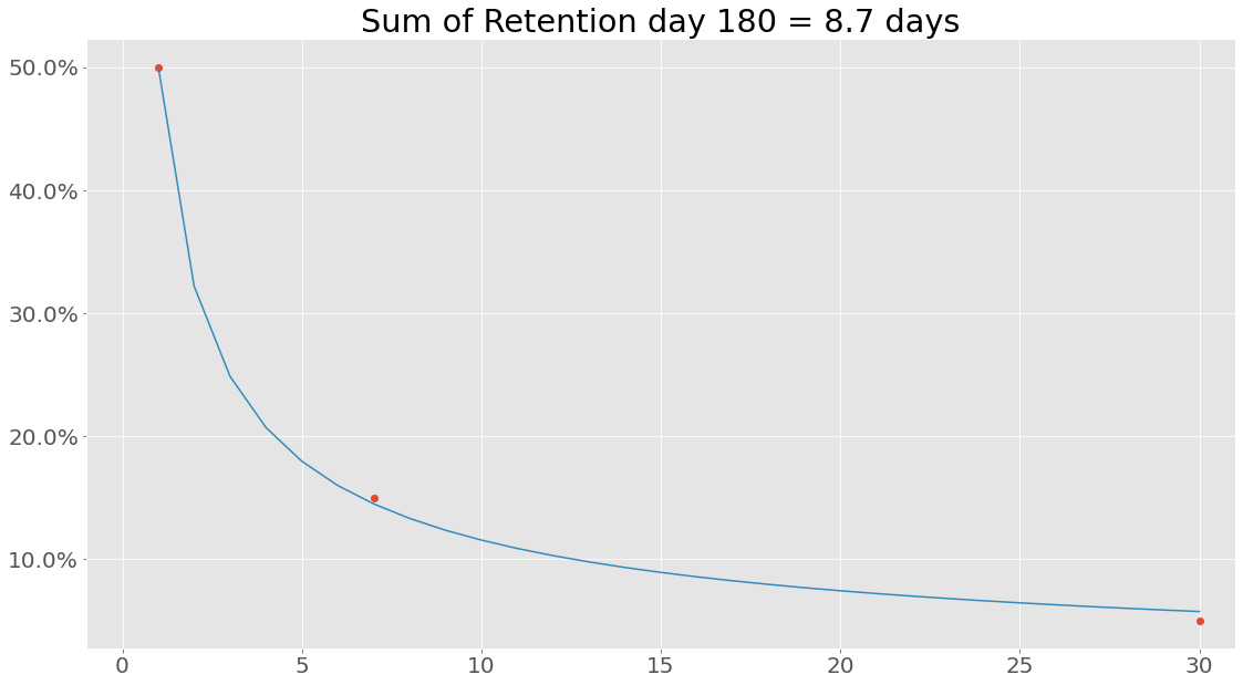
1 50.0%
7 15.0%
30 5.0%
Lets fit an equation to this data, default is a power function and as of right now the only available functions build in are
- Power function: \(f(x) = k_1x^{k_2}\) identifier:
power
Lets see how well it was fitted:
                 Retention RetentionFit
DaysSinceInstall
1                    50.0%        50.1%
2                     nan%        32.2%
3                     nan%        24.9%
4                     nan%        20.7%
5                     nan%        18.0%
6                     nan%        16.0%
7                    15.0%        14.5%
8                     nan%        13.3%
9                     nan%        12.3%
10                    nan%        11.5%
11                    nan%        10.9%
12                    nan%        10.3%
13                    nan%         9.8%
14                    nan%         9.3%
15                    nan%         8.9%
16                    nan%         8.6%
17                    nan%         8.2%
18                    nan%         7.9%
19                    nan%         7.7%
20                    nan%         7.4%
21                    nan%         7.2%
22                    nan%         7.0%
23                    nan%         6.8%
24                    nan%         6.6%
25                    nan%         6.4%
26                    nan%         6.3%
27                    nan%         6.1%
28                    nan%         6.0%
29                    nan%         5.9%
30                    5.0%         5.7%

Let’s try something interesting - what is the sum of the retention values from the retention array?
7.987575025935071
Hmm, that is not the same as the 8.7 calculated using the integrated function of the power equation. At its core the reason for this is that when performing Riemann integration we look at a smooth curve, whereas simply summing retention values from an array we assume a certain linear relationship between point \(R(i)\) and \(R(i+1)\).
Custom Functions
In this example, a power function was used, but any callable function can be used.
NOTE: It is recommended to use the Fitfunction class to create new functions, this class simply needs two functions, the equation used to fit and the integrated equation from 1 to b. The integrated function is only used to calculate the summed retention and can be left out. In that case, just pass the callable function directly. Anyway, example with power function and its integrated companion:
The integral from a to b is simple
Well… Turns out that fitting is not always 100 % similar to real world data, to not get into some bad situations lets set \(a=1\), we can do this, since we know that retention for day 0 is always 1!
Lets create a fitter class for our power function:
Lets fit with this function:
If we are interested in uncertainties the Uncertainties package have been implemented. This can be used the following way:

When working with uncertainties, the nominal values and the uncertainty
values can be obtained with functions nominal_values and
std_devs, respectively:
DaysSinceInstall
1       0.51+/-0.04
2     0.322+/-0.018
3     0.246+/-0.013
4     0.204+/-0.010
5     0.176+/-0.009
6     0.156+/-0.008
7     0.140+/-0.008
8     0.129+/-0.008
9     0.119+/-0.007
10    0.111+/-0.007
11    0.104+/-0.007
12    0.098+/-0.007
13    0.093+/-0.006
14    0.089+/-0.006
15    0.085+/-0.006
16    0.081+/-0.006
17    0.078+/-0.006
18    0.075+/-0.006
19    0.072+/-0.006
20    0.070+/-0.006
21    0.068+/-0.006
22    0.066+/-0.006
23    0.064+/-0.005
24    0.062+/-0.005
25    0.060+/-0.005
26    0.059+/-0.005
27    0.057+/-0.005
28    0.056+/-0.005
29    0.055+/-0.005
30    0.054+/-0.005
Name: RetentionFit, dtype: object
array([0.51007967, 0.32223477, 0.24631593, 0.20356673, 0.17558734,
       0.1556062 , 0.14049706, 0.12860006, 0.11894522, 0.11092453,
       0.10413587, 0.09830176, 0.09322396, 0.0887568 , 0.0847906 ,
       0.08124106, 0.07804224, 0.07514176, 0.07249742, 0.07007482,
       0.06784561, 0.06578619, 0.06387677, 0.06210058, 0.06044333,
       0.05889276, 0.05743829, 0.05607071, 0.054782  , 0.05356512])
array([0.03564148, 0.01775511, 0.01252601, 0.01027747, 0.00909227,
       0.00837123, 0.00788221, 0.00752197, 0.00723962, 0.00700784,
       0.00681092, 0.00663929, 0.00648677, 0.00634921, 0.0062237 ,
       0.00610815, 0.00600099, 0.005901  , 0.00580724, 0.00571896,
       0.00563553, 0.00555645, 0.00548129, 0.00540969, 0.00534132,
       0.00527593, 0.00521327, 0.00515313, 0.00509533, 0.00503971])
So why bother with this integral function anyway? Well, let’s see what happens when we create a data set consisting of retention values from days since install 1 to 180 and sum that using the same power function with the same parameters:
It is also possible to save and load instances of classes (using pickle):
my_retention.save('myretention.pkl')
Loading the data is simply done with
import pyfreya
LoadedRetentionClass = pyfreya.load('myretention.pkl')
Short Tutorial in the Cohort Class.
Retention
Let’s import the class and see insert a some retention numbers along with the amount of new users in the cohort.
To get more info on retenion see retention tutorial.
                        1
DaysSinceInstall
0                     100
1                 50.0629
2                 32.1914
3                 24.8632
4                 20.6996
5                 17.9566
6                 15.9875
7                 14.4921
8                 13.3102
9                  12.348
10                11.5464
11                10.8662
12                10.2802
13                9.76917
14                9.31867
15                8.91795
16                8.55872
17                8.23447
18                7.94001
19                7.67118
20                7.42456
21                7.19733
22                6.98716
23                6.79206
24                6.61038
25                6.44069
26                6.28175
27                6.13252
28                5.99207
29                 5.8596
30                 5.7344
31                5.61586
Note: That the cohort class can also take a retention profile instead of actual retention data points. The name given is not of any particular importance now, but when plotting various aggregates from multiple cohorts easily identifiable names are nice to have - is no name given a random one will be applied.
Daily Active Users
Maybe similar cohorts comes in multiple days in a row. It is moddeled like this:
                       1        2        3        4        5        6        7        8        9        10
DaysSinceInstall
0                     100      100      100      100      100      100      100      100      100      100
1                 50.0629  50.0629  50.0629  50.0629  50.0629  50.0629  50.0629  50.0629  50.0629  50.0629
2                     NaN  32.1914  32.1914  32.1914  32.1914  32.1914  32.1914  32.1914  32.1914  32.1914
3                     NaN      NaN  24.8632  24.8632  24.8632  24.8632  24.8632  24.8632  24.8632  24.8632
4                     NaN      NaN      NaN  20.6996  20.6996  20.6996  20.6996  20.6996  20.6996  20.6996
5                     NaN      NaN      NaN      NaN  17.9566  17.9566  17.9566  17.9566  17.9566  17.9566
6                     NaN      NaN      NaN      NaN      NaN  15.9875  15.9875  15.9875  15.9875  15.9875
7                     NaN      NaN      NaN      NaN      NaN      NaN  14.4921  14.4921  14.4921  14.4921
8                     NaN      NaN      NaN      NaN      NaN      NaN      NaN  13.3102  13.3102  13.3102
9                     NaN      NaN      NaN      NaN      NaN      NaN      NaN      NaN   12.348   12.348
10                    NaN      NaN      NaN      NaN      NaN      NaN      NaN      NaN      NaN  11.5464
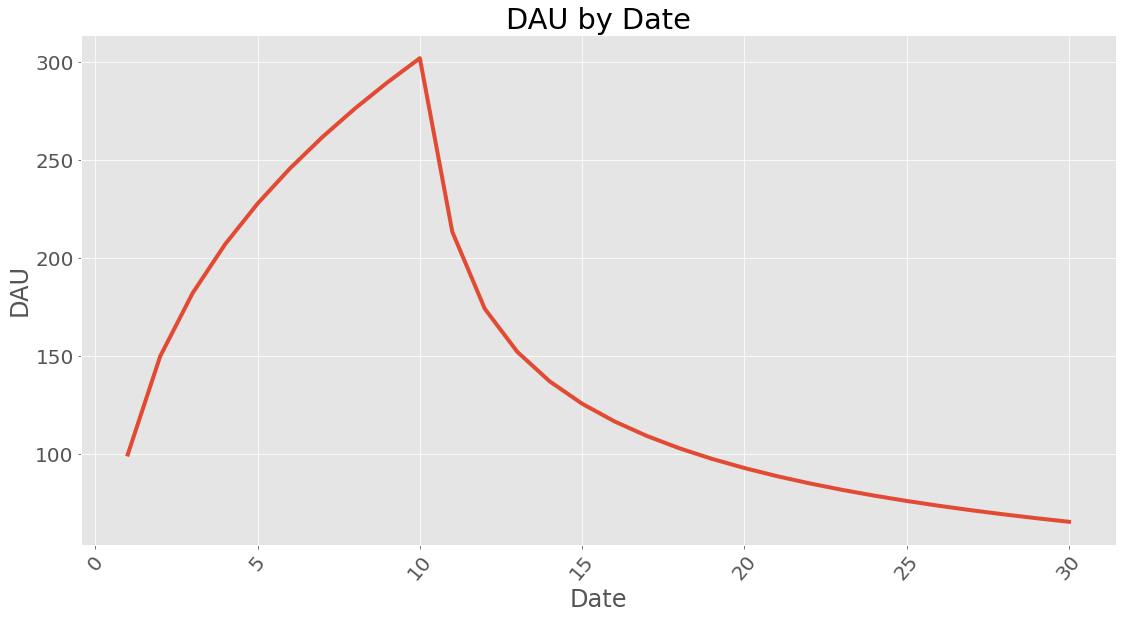
Well - its nice to see this user distribution, but how many daily active users do we have ? (also note the type is a pandas DataFrame)
<class 'pandas.core.frame.DataFrame'>
| dau | |
|---|---|
| Date | |
| 1 | 100 |
| 2 | 150.063 |
| 3 | 182.254 |
| 4 | 207.117 |
| 5 | 227.817 |
| 6 | 245.774 |
| 7 | 261.761 |
| 8 | 276.253 |
| 9 | 289.563 |
| 10 | 301.912 |
Since users are still active after the influx of 10 days lets see what it looks like after 30 days (10 days of user influx and 20 days of waiting):
| dau | |
|---|---|
| Date | |
| 1 | 100 |
| 2 | 150.063 |
| 3 | 182.254 |
| 4 | 207.117 |
| 5 | 227.817 |
| 6 | 245.774 |
| 7 | 261.761 |
| 8 | 276.253 |
| 9 | 289.563 |
| 10 | 301.912 |
| 11 | 213.458 |
| 12 | 174.261 |
| 13 | 152.35 |
| 14 | 137.256 |
| 15 | 125.875 |
| 16 | 116.836 |
| 17 | 109.408 |
| 18 | 103.15 |
| 19 | 97.7799 |
| 20 | 93.103 |
| 21 | 88.9812 |
| 22 | 85.3123 |
| 23 | 82.0192 |
| 24 | 79.0421 |
| 25 | 76.3338 |
| 26 | 73.8566 |
| 27 | 71.5796 |
| 28 | 69.4776 |
| 29 | 67.5297 |
| 30 | 65.7181 |
Enough numbers, lets plot some of this. First, lets plot the retention - maybe it fitted the data incorrectly:

How about dau?
If you wonder how long time it takes to reach a certain amount of dau it can be calculated. This does assume a steady influx of users given in new_users and with the retention profile calculated earlier.
21
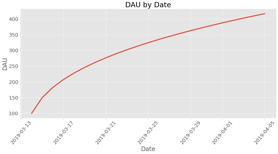
Datetime
What kind of date is this anyway? Lets use proper human dates from the Gregorian calendar:
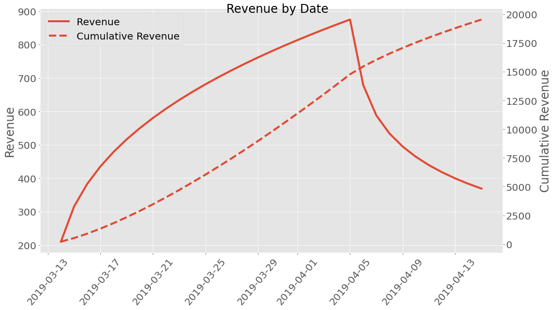
Revenue
Well how much money did we earn? A premade revenue profile class called
ARPDAU is imported and is initialized by setting the ARPDAU to a
value.
| dau | revenue | |
|---|---|---|
| Date | ||
| 2019-03-14 | 100 | 210 |
| 2019-03-15 | 150.063 | 315.132 |
| 2019-03-16 | 182.254 | 382.734 |
| 2019-03-17 | 207.117 | 434.947 |
| 2019-03-18 | 227.817 | 478.416 |
| 2019-03-19 | 245.774 | 516.125 |
| 2019-03-20 | 261.761 | 549.698 |
| 2019-03-21 | 276.253 | 580.132 |
| 2019-03-22 | 289.563 | 608.083 |
| 2019-03-23 | 301.912 | 634.014 |
| 2019-03-24 | 313.458 | 658.262 |
| 2019-03-25 | 324.324 | 681.081 |
| 2019-03-26 | 334.604 | 702.669 |
| 2019-03-27 | 344.374 | 723.184 |
| 2019-03-28 | 353.692 | 742.754 |
| 2019-03-29 | 362.61 | 761.481 |
| 2019-03-30 | 371.169 | 779.455 |
| 2019-03-31 | 379.403 | 796.747 |
| 2019-04-01 | 387.343 | 813.421 |
| 2019-04-02 | 395.015 | 829.531 |
| 2019-04-03 | 402.439 | 845.122 |
| 2019-04-04 | 409.636 | 860.237 |
| 2019-04-05 | 416.624 | 874.91 |
| 2019-04-06 | 323.416 | 679.173 |
| 2019-04-07 | 279.963 | 587.923 |
| 2019-04-08 | 254.212 | 533.846 |
| 2019-04-09 | 235.631 | 494.825 |
| 2019-04-10 | 221.064 | 464.234 |
| 2019-04-11 | 209.099 | 439.109 |
| 2019-04-12 | 198.971 | 417.84 |
| 2019-04-13 | 190.214 | 399.449 |
| 2019-04-14 | 182.519 | 383.291 |
| 2019-04-15 | 175.675 | 368.917 |
This can be plotted too!
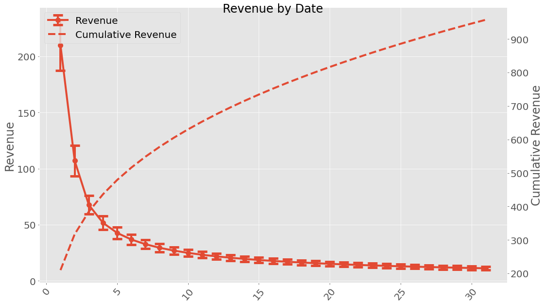
If we are interested in uncertainties the Uncertainties package have been implemented. This can be used the following way:
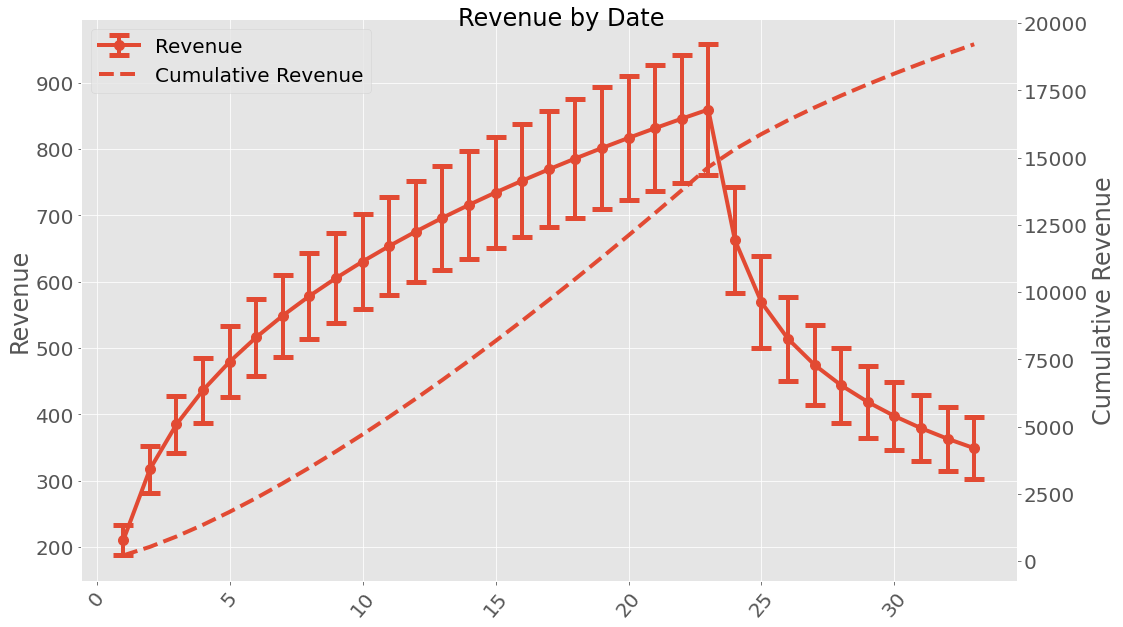
When working with uncertainties, the nominal values and the uncertainty
values can be obtained with functions nominal_values and
std_devs, respectively:
Date
1      100+/-5
2      151+/-8
3     183+/-11
4     208+/-12
5     228+/-14
6     246+/-15
7     261+/-16
8     275+/-17
9     288+/-17
10    300+/-18
11    311+/-19
12    322+/-20
13    331+/-20
14    341+/-21
15    350+/-22
16    358+/-22
17    366+/-23
18    374+/-23
19    382+/-24
20    389+/-24
21    396+/-25
22    403+/-26
23    409+/-26
24    316+/-23
25    271+/-21
26    245+/-19
27    226+/-19
28    211+/-18
29    199+/-17
30    189+/-17
31    181+/-16
32    173+/-16
33    166+/-16
Name: dau, dtype: object
array([100.        , 151.00796688, 183.23144399, 207.86303692,
       228.21970943, 245.77844367, 261.3390633 , 275.38876963,
       288.24877584, 300.14329757, 311.23575048, 321.64933796,
       331.47951354, 340.80190942, 349.6775894 , 358.15664906,
       366.28075478, 374.08497899, 381.59915514, 388.84889718,
       395.85637904, 402.64093973, 409.21955908, 315.60723627,
       270.8093275 , 244.6301836 , 225.88786696, 211.27502302,
       199.32335936, 189.24093946, 180.54774509, 172.92912575,
       166.16687945])
array([ 5.        ,  8.34935123, 10.56825389, 12.20066331, 13.51786087,
       14.6418741 , 15.63646161, 16.53872917, 17.37200759, 18.15183883,
       18.88905055, 19.59146105, 20.26488384, 20.91374916, 21.54150443,
       22.1508812 , 22.74407817, 23.32289008, 23.88880016, 24.44304807,
       24.98668034, 25.52058868, 26.04553928, 22.86365271, 20.63415691,
       19.40634919, 18.5255104 , 17.82742722, 17.24464372, 16.74232945,
       16.29990806, 15.90409195, 15.54574024])
It is possible to save a cohort class instance (using pickle) and loading it.
facebook.save('facebook_revenue.pkl')
import pyfreya
facebook_loaded = pyfreya.load('facebook_revenue.pkl')
Short Tutorial in the Revenue Classes.
Let’s import the class and insert a some retention numbers along with the amount of new users in a cohort. Additional information about Retention and Cohort classes can be found at retention tutorial and cohort tutorial. Let’s also import a predefined revenue spending class (profile) ARPDAU.
                        1
DaysSinceInstall
0                     100
1                 50.0629
2                 32.1914
3                 24.8632
4                 20.6996
5                 17.9566
6                 15.9875
7                 14.4921
8                 13.3102
9                  12.348
10                11.5464
11                10.8662
12                10.2802
13                9.76917
14                9.31867
15                8.91795
16                8.55872
17                8.23447
18                7.94001
19                7.67118
20                7.42456
21                7.19733
22                6.98716
23                6.79206
24                6.61038
25                6.44069
26                6.28175
27                6.13252
28                5.99207
29                 5.8596
30                 5.7344
31                5.61586
| dau | revenue | |
|---|---|---|
| Date | ||
| 1 | 100 | 210 |
| 2 | 50.0629 | 105.132 |
| 3 | 32.1914 | 67.6019 |
| 4 | 24.8632 | 52.2127 |
| 5 | 20.6996 | 43.4692 |
| 6 | 17.9566 | 37.7089 |
| 7 | 15.9875 | 33.5737 |
| 8 | 14.4921 | 30.4334 |
| 9 | 13.3102 | 27.9515 |
| 10 | 12.348 | 25.9309 |
| 11 | 11.5464 | 24.2475 |
| 12 | 10.8662 | 22.819 |
| 13 | 10.2802 | 21.5885 |
| 14 | 9.76917 | 20.5153 |
| 15 | 9.31867 | 19.5692 |
| 16 | 8.91795 | 18.7277 |
| 17 | 8.55872 | 17.9733 |
| 18 | 8.23447 | 17.2924 |
| 19 | 7.94001 | 16.674 |
| 20 | 7.67118 | 16.1095 |
| 21 | 7.42456 | 15.5916 |
| 22 | 7.19733 | 15.1144 |
| 23 | 6.98716 | 14.673 |
| 24 | 6.79206 | 14.2633 |
| 25 | 6.61038 | 13.8818 |
| 26 | 6.44069 | 13.5254 |
| 27 | 6.28175 | 13.1917 |
| 28 | 6.13252 | 12.8783 |
| 29 | 5.99207 | 12.5833 |
| 30 | 5.8596 | 12.3052 |
| 31 | 5.7344 | 12.0422 |
As can be seen, there is also room for adding uncertainty. Let’s import
the base revenue class and define ARPDAU but with uncertainty. It does
make use of some properties of the Cohort class, it is recommended
to be a bit familiar with that.
| dau | revenue | |
|---|---|---|
| Date | ||
| 1 | 100 | 210 |
| 2 | 50.0629 | 105.132 |
| 3 | 32.1914 | 67.6019 |
| 4 | 24.8632 | 52.2127 |
| 5 | 20.6996 | 43.4692 |
| 6 | 17.9566 | 37.7089 |
| 7 | 15.9875 | 33.5737 |
| 8 | 14.4921 | 30.4334 |
| 9 | 13.3102 | 27.9515 |
| 10 | 12.348 | 25.9309 |
| 11 | 11.5464 | 24.2475 |
| 12 | 10.8662 | 22.819 |
| 13 | 10.2802 | 21.5885 |
| 14 | 9.76917 | 20.5153 |
| 15 | 9.31867 | 19.5692 |
| 16 | 8.91795 | 18.7277 |
| 17 | 8.55872 | 17.9733 |
| 18 | 8.23447 | 17.2924 |
| 19 | 7.94001 | 16.674 |
| 20 | 7.67118 | 16.1095 |
| 21 | 7.42456 | 15.5916 |
| 22 | 7.19733 | 15.1144 |
| 23 | 6.98716 | 14.673 |
| 24 | 6.79206 | 14.2633 |
| 25 | 6.61038 | 13.8818 |
| 26 | 6.44069 | 13.5254 |
| 27 | 6.28175 | 13.1917 |
| 28 | 6.13252 | 12.8783 |
| 29 | 5.99207 | 12.5833 |
| 30 | 5.8596 | 12.3052 |
| 31 | 5.7344 | 12.0422 |
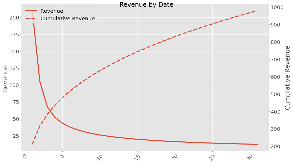
If we are interested in uncertainties the Uncertainties package have been implemented. This can be used the following way:
When working with uncertainties, the nominal values and the uncertainty
values can be obtained with functions nominal_values and
std_devs, respectively:
Date
1       210+/-23
2       107+/-14
3         68+/-8
4         52+/-6
5         43+/-5
6         37+/-4
7         33+/-4
8         30+/-4
9     27.0+/-3.3
10    25.0+/-3.1
11    23.3+/-2.9
12    21.9+/-2.8
13    20.6+/-2.6
14    19.6+/-2.5
15    18.6+/-2.4
16    17.8+/-2.3
17    17.1+/-2.2
18    16.4+/-2.2
19    15.8+/-2.1
20    15.2+/-2.0
21    14.7+/-2.0
22    14.2+/-1.9
23    13.8+/-1.9
24    13.4+/-1.8
25    13.0+/-1.8
26    12.7+/-1.8
27    12.4+/-1.7
28    12.1+/-1.7
29    11.8+/-1.7
30    11.5+/-1.6
31    11.2+/-1.6
Name: revenue, dtype: object
array([210.        , 107.11673044,  67.66930193,  51.72634515,
        42.74901227,  36.8733419 ,  32.67730124,  29.50438329,
        27.00601304,  24.97849563,  23.29415112,  21.86853369,
        20.64336873,  19.57703135,  18.63892795,  17.80602528,
        17.06062202,  16.38887082,  15.77976993,  15.22445827,
        14.71571191,  14.24757745,  13.81510062,  13.41412211,
        13.04112202,  12.69309974,  12.36748022,  12.06203999,
        11.77484823,  11.50421944,  11.24867512])
array([22.588714  , 13.73966474,  8.17827559,  6.15442801,  5.07962406,
        4.40195366,  3.9300445 ,  3.57937697,  3.3066122 ,  3.08712987,
        2.90585349,  2.75300466,  2.62194609,  2.5080031 ,  2.40778109,
        2.31875073,  2.23898552,  2.16699004,  2.1015841 ,  2.04182268,
        1.9869392 ,  1.93630468,  1.88939763,  1.84578168,  1.80508855,
        1.76700502,  1.73126286,  1.69763082,  1.66590837,  1.63592067,
        1.60751445])
It is possible to save a revenue class instance (using pickle) and loading it.
facebook.save('facebook_revenue.pkl')
facebook_loaded = pyfreya.load('facebook_revenue.pkl')
Short Tutorial Working With Multiple Cohorts
When working with multiple cohorts plotting can’t be performed with the Cohort class methods, instead, import multi plot functions. Let’s create some cohorts first.
Lets plot their retention

If copies of the Facebook cohort comes in each day in 10 days and copies of the Google cohort comes in 6 days in a row - what does DAU look like?


How does revenue look across this? Lets apply a revenue profile and take a look.


If we are interested in uncertainties the Uncertainties package have been implemented. This can be used the following way:


When working with uncertainties, the nominal values and the uncertainty
values can be obtained with functions nominal_values and
std_devs, respectively:
Date
1      100+/-6
2     152+/-10
3     185+/-13
4     209+/-16
5     230+/-17
6     247+/-19
7     262+/-20
8     276+/-21
9     288+/-22
10    300+/-23
Name: dau, dtype: object
array([100.        , 152.2302569 , 184.70997132, 209.30960342,
       229.50731853, 246.84077882, 262.13821507, 275.9019684 ,
       288.46204483, 300.04808586])
array([ 6.        , 10.49918186, 13.4983251 , 15.64446572, 17.31653098,
       18.69011938, 19.85918453, 20.87961789, 21.78730166, 22.60661843])