pyfreya.retention package
Submodules
pyfreya.retention.fit_functions module
Class for functions to fit
-
class
pyfreya.retention.fit_functions.BaseFitFunction(fit_func, integrate_func)[source]¶ Bases:
objectBase class for fit functions.
-
integrate(b=180, **kwargs)[source]¶ Calculates the integral of the fit function from a constant (suggested is 1) to b. Additional arguments are parameter values.
Parameters: - b – Last day since install value.
- kwargs – Parameter values.
Return type: floatReturns: Integrated value over the fit function.
-
pyfreya.retention.retention module
Short Tutorial in the Retention Class.
Let’s import the class and see insert a some retention numbers.
Lets see what what we have in here:
                 Retention
DaysSinceInstall
1                    50.0%
7                    15.0%
30                    5.0%
Lets fit an equation to this data, default is a power function and as of right now the only available functions build in are
- Power function: \(f(x) = k_1x^{k_2}\) identifier:
power
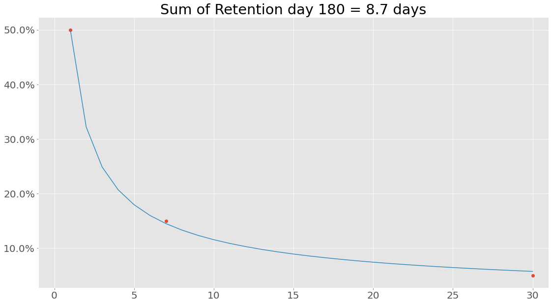
Lets see how well it was fitted:
                 Retention RetentionFit
DaysSinceInstall
1                    50.0%        50.1%
2                     nan%        32.2%
3                     nan%        24.9%
4                     nan%        20.7%
5                     nan%        18.0%
6                     nan%        16.0%
7                    15.0%        14.5%
8                     nan%        13.3%
9                     nan%        12.3%
10                    nan%        11.5%
11                    nan%        10.9%
12                    nan%        10.3%
13                    nan%         9.8%
14                    nan%         9.3%
15                    nan%         8.9%
16                    nan%         8.6%
17                    nan%         8.2%
18                    nan%         7.9%
19                    nan%         7.7%
20                    nan%         7.4%
21                    nan%         7.2%
22                    nan%         7.0%
23                    nan%         6.8%
24                    nan%         6.6%
25                    nan%         6.4%
26                    nan%         6.3%
27                    nan%         6.1%
28                    nan%         6.0%
29                    nan%         5.9%
30                    5.0%         5.7%

Let’s try something interesting - what is the sum of the retention values from the retention array?
7.987575025935071
Hmm, that is not the same as the 8.7 calculated using the integrated function of the power equation. At its core the reason for this is that when performing Riemann integration we look at a smooth curve, whereas simply summing retention values from an array we assume a certain linear relationship between point \(R(i)\) and \(R(i+1)\).
Custom Functions
In this example, a power function was used, but any callable function can be used.
NOTE: It is recommended to use the Fitfunction class to create new functions, this class simply needs two functions, the equation used to fit and the integrated equation from 1 to b. The integrated function is only used to calculate the summed retention and can be left out. In that case, just pass the callable function directly. Anyway, example with power function and its integrated companion:
The integral from a to b is simple
Well… Turns out that fitting is not always 100 % similar to real world data, to not get into some bad situations lets set \(a=1\), we can do this, since we know that retention for day 0 is always 1!
Lets create a fitter class for our power function:
Lets fit with this function:
If we are interested in uncertainties the Uncertainties package have been implemented. This can be used the following way:
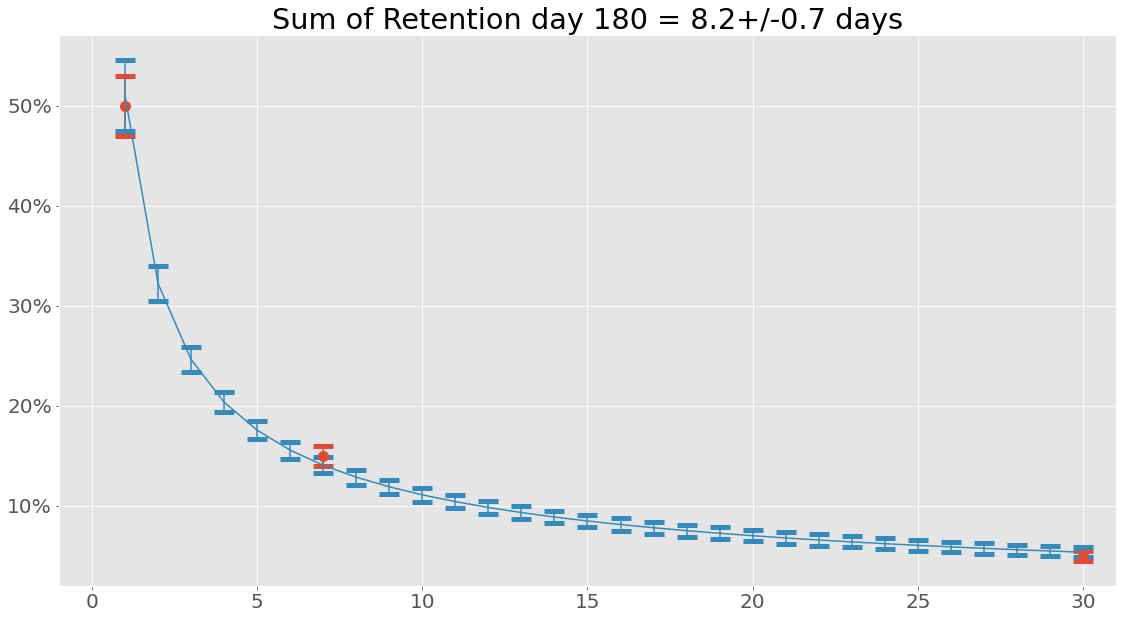
When working with uncertainties, the nominal values and the uncertainty
values can be obtained with functions nominal_values and
std_devs, respectively:
DaysSinceInstall
1       0.51+/-0.04
2     0.322+/-0.018
3     0.246+/-0.013
4     0.204+/-0.010
5     0.176+/-0.009
6     0.156+/-0.008
7     0.140+/-0.008
8     0.129+/-0.008
9     0.119+/-0.007
10    0.111+/-0.007
11    0.104+/-0.007
12    0.098+/-0.007
13    0.093+/-0.006
14    0.089+/-0.006
15    0.085+/-0.006
16    0.081+/-0.006
17    0.078+/-0.006
18    0.075+/-0.006
19    0.072+/-0.006
20    0.070+/-0.006
21    0.068+/-0.006
22    0.066+/-0.006
23    0.064+/-0.005
24    0.062+/-0.005
25    0.060+/-0.005
26    0.059+/-0.005
27    0.057+/-0.005
28    0.056+/-0.005
29    0.055+/-0.005
30    0.054+/-0.005
Name: RetentionFit, dtype: object
array([0.51007967, 0.32223477, 0.24631593, 0.20356673, 0.17558734,
       0.1556062 , 0.14049706, 0.12860006, 0.11894522, 0.11092453,
       0.10413587, 0.09830176, 0.09322396, 0.0887568 , 0.0847906 ,
       0.08124106, 0.07804224, 0.07514176, 0.07249742, 0.07007482,
       0.06784561, 0.06578619, 0.06387677, 0.06210058, 0.06044333,
       0.05889276, 0.05743829, 0.05607071, 0.054782  , 0.05356512])
array([0.03564148, 0.01775511, 0.01252601, 0.01027747, 0.00909227,
       0.00837123, 0.00788221, 0.00752197, 0.00723962, 0.00700784,
       0.00681092, 0.00663929, 0.00648677, 0.00634921, 0.0062237 ,
       0.00610815, 0.00600099, 0.005901  , 0.00580724, 0.00571896,
       0.00563553, 0.00555645, 0.00548129, 0.00540969, 0.00534132,
       0.00527593, 0.00521327, 0.00515313, 0.00509533, 0.00503971])
So why bother with this integral function anyway? Well, let’s see what happens when we create a data set consisting of retention values from days since install 1 to 180 and sum that using the same power function with the same parameters:
It is also possible to save and load instances of classes (using pickle):
my_retention.save('myretention.pkl')
Loading the data is simply done with
import pyfreya
LoadedRetentionClass = pyfreya.load('myretention.pkl')
Retention Class
-
class
pyfreya.retention.retention.Retention(days_since_install, retention_values)[source]¶ Bases:
objectRetention class Start
-
fit(function='power', **kwargs)[source]¶ Fits given values to a function. function can either be an identifier (string) of these:
- power: Calls a power function.
function can also be a custom callable function. Additional arguments can be passed to scipy s curve fitting tool: curve fitting function
Parameters: function ( Union[str,Callable]) – String (identifier) or callable function.Returns: 0
-
retention_sum(dsi_end=180)[source]¶ Calculates the sum of retention (mean average days the game have been opened at least once). It uses the parameters from a fit to calculate it and is only possible if the fit function is of the
BaseFitFunctionclass.Parameters: dsi_end – The last day in the integration. Return type: floatReturns: Sum of retention.
-
Module contents
inits retention